About the Technique

Although regression has been around for a very long time, advances in computing have catapulted it into the world of “machine learning” for business applications.

Linear regression is a basic statistical technique that can be used to predict how many units you are likely to sell based on a given price. With that information a business can also take things a step further by adding cost into the mix and then determine what price is most likely to maximize profits. In other words linear models can help take guesswork out of price setting.

There are a lot of nuances in regression models, but for something simple like quantity predicted by price you can do the job in Microsoft Excel quite easily with a few mouse clicks, no need to even write a formula.

Simple Regression in Microsoft Excel

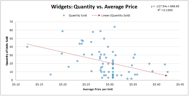This can be accomplished by creating two columns to use with a scatterplot, price and quantity sold. Then on the resulting graph you simply right click on one of the points and select “add trend line.” Make sure to choose a linear model. While you are at it is helpful to double-click the trendline and add checkboxes for showing the formula and R2 value.

This formula (y=-127.54x + 696.93) can then be used to estimate quantity sold for any given price: Quantity Sold is estimated to be -127.54 multiplied by Price plus 696.93. However, R2 lets you know that price only explains 15% of the variation in the data, so the model is not very accurate. More specifically we could say that price is a weak predictor of demand over the available range, or not a large factor in purchasing decisions when it is near $5.25 per unit.

This analysis can easily be performed in a few minutes by anyone with a copy of Excel. Immediately we can tell that price does not play a large role in purchase decisions because of the low R2 score and the plot looks like “cloud” of data. However, visually it does appear that quantity sold drops after $5.35 so we want to tread carefully there with an eye on our competition.

A bit of Caution

A word of caution, the time period you choose for measurement is important. It may be wise to aggregate data weekly to remove fluctuations between high volume and low volume days and use an average weekly price. Similarly, removing extreme values that are clearly skewing the trend line is a good idea. These can be deleted or replaced with the median values for the analysis.

It is also worth a mention that items with extreme seasonal swings such as fruit or ski equipment are better handled with time-series techniques (not covered in this article). For these products the current season is often better predictor of unit volumes than price.

Price Optimization

Trying to predict the optimal price over a 20 cent range with a weakly correlated model is probably not worth the effort, suffice to say that the price appears fine around $5.25 +/- and lowering it seems unlikely to significantly boost our volume. In other words, the price seems fair to consumers, but we need another strategy if our goal is increasing volume.

While these simple models provide helpful insights, the decision on pricing is ultimately still a human one. It is generally a good idea to set the price based on willingness to pay as the first consideration, and cost or volume as secondary considerations. However, if you find yourself wondering how to measure willingness to pay in the real world, simple linear regression may offer the solution.